A 038 Kg Pendulum Bob Is Attached to a String 12 M Long You May Want to Review

Lab 7 - Simple Harmonic Motion

Introduction

Have you always wondered why a grandad clock keeps authentic time? The movement of the pendulum is a detail kind of repetitive or periodic motion called simple harmonic motion, or SHM. The position of the oscillating object varies sinusoidally with fourth dimension. Many objects oscillate dorsum and forth. The motion of a child on a swing tin can be approximated to be sinusoidal and tin can therefore exist considered as elementary harmonic motion. Some complicated motions similar turbulent water waves are not considered simple harmonic motion. When an object is in simple harmonic movement, the rate at which it oscillates back and forth as well as its position with respect to fourth dimension tin be hands determined. In this lab, you volition analyze a simple pendulum and a bound-mass system, both of which exhibit simple harmonic motion.

Discussion of Principles

A particle that vibrates vertically in simple harmonic motility moves upwardly and downwardly between two extremes y = ±A. The maximum deportation A is chosen the amplitude. This motion is shown graphically in the position-versus-time plot in Fig. 1.

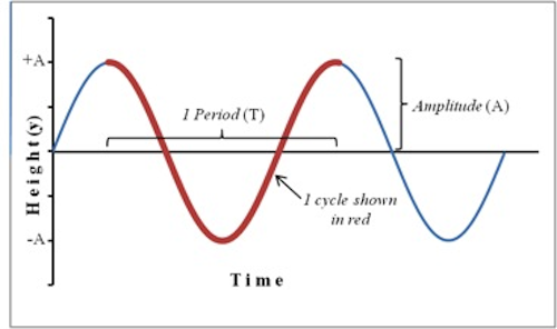
Figure 1 : Position plot showing sinusoidal motility of an object in SHM

One complete oscillation or bike or vibration is the motion from, for case,

y = − A

to

y = + A

and back again to

y = − A .

The time interval T required to complete one oscillation is called the period. A related quantity is the frequency f, which is the number of vibrations the arrangement makes per unit of time. The frequency is the reciprocal of the menses and is measured in units of Hertz, abbreviated Hz;

1 Hz = 1 s⁻¹.

If a particle is aquiver along the y-axis, its location on the y-centrality at whatsoever given instant of time t, measured from the start of the oscillation is given past the equation

Recall that the velocity of the object is the first derivative and the dispatch the second derivative of the deportation office with respect to time. The velocity v and the dispatch a of the particle at time t are given by

( 4 )

a = −(2π f )²[ A sin(2π ft )]

Notice that the velocity and acceleration are as well sinusoidal. Yet the velocity role has a ninety° or π/two stage deviation while the dispatch function has a 180° or π phase divergence relative to the displacement function. For example, when the deportation is positive maximum, the velocity is zero and the acceleration is negative maximum. Substituting from Eq. (1)

f = 1/ T

into Eq. (4)

a = −(2π f )²[ A sin(2π ft )]

yields From Eq. (5)

a = −4π ² f ² y

nosotros come across that the acceleration of an object in SHM is proportional to the displacement and reverse in sign. This is a bones property of whatsoever object undergoing uncomplicated harmonic motility. Consider several critical points in a bicycle as in the case of a spring-mass arrangement in oscillation. A spring-mass system consists of a mass fastened to the stop of a spring that is suspended from a stand. The mass is pulled down by a small amount and released to make the spring and mass oscillate in the vertical plane. Effigy ii shows 5 critical points as the mass on a spring goes through a complete wheel. The equilibrium position for a leap-mass system is the position of the mass when the leap is neither stretched nor compressed.

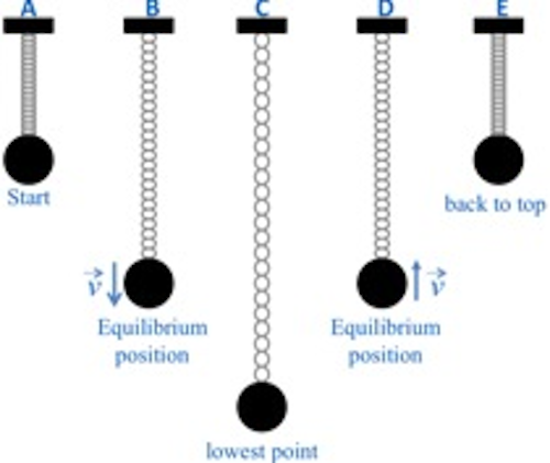
Effigy 2 : Five central points of a mass oscillating on a spring.

The mass completes an unabridged bike every bit information technology goes from position A to position East. A clarification of each position is as follows:

• Position A: The spring is compressed; the mass is in a higher place the equilibrium point at

  y = A

  and is nearly to be released.
• Position B: The mass is in downward motion every bit it passes through the equilibrium point.
• Position C: The mass is momentarily at residual at the lowest point before starting on its upward movement.
• Position D: The mass is in upwards motion as it passes through the equilibrium point.
• Position Due east: The mass is momentarily at rest at the highest point before starting back downward over again.

By noting the time when the negative maximum, positive maximum, and zero values occur for the aquiver object's position, velocity, and acceleration, you can graph the sine (or cosine) office. This is done for the instance of the oscillating spring-mass system in the table beneath and the three functions are shown in Fig. 3. Notation that the positive direction is typically chosen to be the direction that the spring is stretched. Therefore, the positive direction in this case is down and the initial position A in Fig. ii is actually a negative value. The most difficult parameter to analyze is the acceleration. It helps to utilise Newton's second police force, which tells us that a negative maximum acceleration occurs when the internet force is negative maximum, a positive maximum dispatch occurs when the net force is positive maximum and the acceleration is zero when the internet force is zero.

	Position	Velocity	Dispatch
Indicate A	neg max	zippo	pos max
Point B	zero	pos max	nil
Betoken C	pos max	nada	neg max
Betoken D	nothing	neg max	zero
Signal E	neg max	nada	pos max

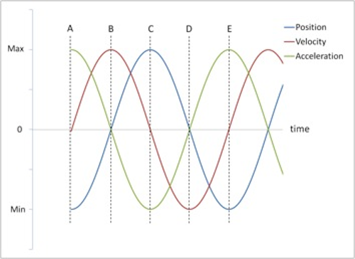
Figure 3 : Position, velocity and acceleration vs. fourth dimension

For this particular initial status (starting position at A in Fig. 2), the position curve is a cosine function (really a negative cosine role), the velocity curve is a sine function, and the dispatch curve is just the negative of the position bend.

Mass and Spring

A mass suspended at the end of a spring will stretch the spring by some altitude y. The forcefulness with which the spring pulls upward on the mass is given by Hooke's law where 1000 is the spring constant and y is the stretch in the leap when a strength F is applied to the leap. The leap abiding grand is a mensurate of the stiffness of the spring. The spring abiding can exist determined experimentally past assuasive the mass to hang motionless on the leap and and then calculation additional mass and recording the boosted spring stretch as shown below. In Fig. 4a the weight hanger is suspended from the end of the spring. In Fig. 4b, an additional mass has been added to the hanger and the spring is now extended past an amount

Δ y

. This experimental set-up is likewise shown in the photograph of the appliance in Fig. 5.

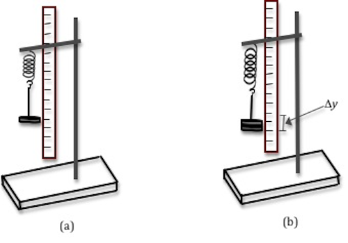
Figure iv : Ready for determining spring constant

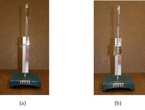
Figure 5 : Photo of set up-up for determining spring constant

When the mass is motionless, its acceleration is zero. According to Newton'southward 2d law the net forcefulness must therefore be zippo. At that place are ii forces acting on the mass; the downwardly gravitational force and the up leap force. See the free-body diagram in Fig. half-dozen beneath.

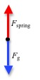
Figure half dozen : Free-body diagram for the spring-mass system

Then Newton's second law gives us where

Δ k

is the alter in mass and

Δ y

is the change in the stretch of the spring caused by the modify in mass, 1000 is the gravitational acceleration, and yard is the jump constant. Eq. (seven)

Δ mg − m Δ y = 0

tin besides be expressed every bit Newton's 2nd law applied to this system is

ma = F = − ky .

Substitute from Eq. (5)

a = −fourπ ² f ² y

for the acceleration to go from which nosotros become an expression for the frequency f and the catamenia T.

( ten )

f =

( 11 )

T = twoπ

Using Eq. (xi)

T = 2π

we can predict the catamenia if we know the mass on the spring and the spring abiding. Alternately, knowing the mass on the spring and experimentally measuring the menses, nosotros tin determine the spring abiding of the spring. Notice that in Eq. (11)

T = 2π

the relationship between T and thousand is not linear. A graph of the menstruum versus the mass will not be a straight line. If we foursquare both sides of Eq. (eleven)

T = 2π

, we get Now a graph of

T ^two

versus chiliad will be a directly line and the jump constant can be determined from the slope.

Simple Pendulum

The other example of elementary harmonic motion that you will investigate is the simple pendulum. The simple pendulum consists of a mass m, called the pendulum bob, attached to the end of a cord. The length L of the simple pendulum is measured from the signal of break of the cord to the center of the bob equally shown in Fig. vii beneath.

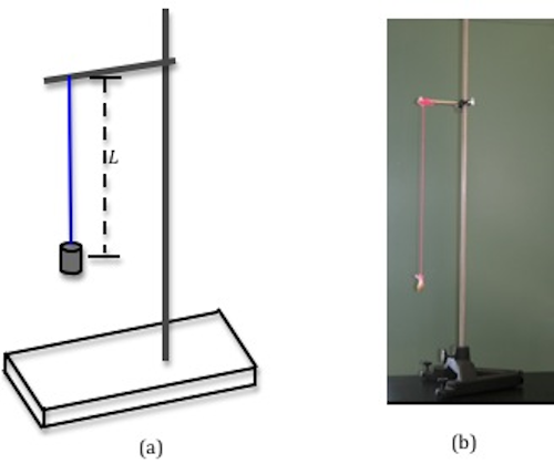
Figure 7 : Experimental ready-up for a uncomplicated pendulum

If the bob is moved away from the rest position through some angle of displacement θ as in Fig. 7, the restoring forcefulness volition return the bob dorsum to the equilibrium position. The forces acting on the bob are the strength of gravity and the tension force of the string. The tension strength of the string is counterbalanced past the component of the gravitational force that is in line with the string (i.due east. perpendicular to the motion of the bob). The restoring strength here is the tangential component of the gravitational strength.

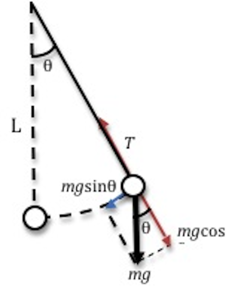
Effigy viii : Simple pendulum

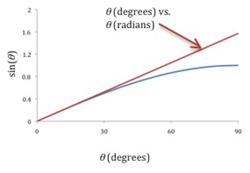
When we utilise trigonometry to the smaller triangle in Fig. eight, we get the magnitude of the restoring force

| F | = mg sin θ.

This forcefulness depends on the mass of the bob, the acceleration due to gravity m and the sine of the angle through which the string has been pulled. Again Newton'due south second law must apply, and so

( xiii )

ma = F = − mg sin θ

where the negative sign implies that the restoring force acts opposite to the direction of motion of the bob. Since the bob is moving along the arc of a circumvolve, the angular acceleration is given by

α = a / Fifty .

From Eq. (thirteen)

ma = F = − mg sin θ

we get In Fig. 9 the blue solid line is a plot of θ versus sin(θ) and the straight line is a plot of θ in degrees versus θ in radians. For small angles these ii curves are nearly indistinguishable. Therefore, as long as the displacement θ is small nosotros can utilise the approximation sin θ ≅ θ.

Effigy 9 : Graphs of sin θ versus θ

With this approximation Eq. (14)

α = − sin θ

becomes Equation (15) shows the (angular) dispatch to be proportional to the negative of the (athwart) displacement and therefore the motion of the bob is unproblematic harmonic and we can use Eq. (5)

a = −4π ² f ² y

to get Combining Eq. (15)

α = − θ

and Eq. (sixteen)

α = −4π ^two f ² θ

, and simplifying, we become

( 17 )

f =

and

( eighteen )

T = iiπ

Note that the frequency and period of the simple pendulum practice not depend on the mass.

Objective

The objective of this lab is to sympathise the behavior of objects in elementary harmonic motion by determining the spring abiding of a bound-mass system and a simple pendulum.

Equipment

• Assorted masses
• Bound
• Meter stick
• Stand up
• Stopwatch
• String
• Pendulum bob
• Protractor
• Balance

Procedure

Using Hooke'due south police force you will determine the spring constant of the spring by measuring the jump stretch as boosted masses are added to the jump. You will determine the period of oscillation of the spring-mass organization for unlike masses and apply this to determine the spring constant. Yous will then compare the leap constant values obtained by the ii methods. In the case of the simple pendulum, you will measure out the period of oscillation for varying lengths of the pendulum string and compare these values to the predicted values of the period.

Procedure A: Determining Jump Constant Using Hooke'due south Constabulary

• 1

  Starting with 50 one thousand, add masses in steps of 50 g to the hanger. As you add each 50 g mass, mensurate the corresponding elongation y of the spring produced by the weight of these added masses. Enter these values in Data Tabular array 1.

• 2

  Use Excel to plot m versus y. Come across Appendix G.

• 3

  Use the trendline option in Excel to determine the slope of the graph. Record this value on the worksheet. Run into Appendix H.

• 4

  Use the value of the slope to determine the spring abiding k of the spring. Record this value on the worksheet.

Checkpoint 1:
Ask your TA to cheque your table and Excel graph.

Procedure B: Determining Jump Constant from

T ⁱⁱ

vs. grand Graph

We have causeless the spring to exist massless, but information technology has some mass, which will affect the menses of oscillation. Theory predicts and feel verifies that if one-tertiary the mass of the spring were added to the mass m in Eq. (11)

T = iiπ

, the menstruation will be the same as that of a mass of this full magnitude, aquiver on a massless spring.

• five

  Utilize the residuum to measure the mass of the bound and record this on the worksheet. Add one-3rd this mass to the aquiver mass before calculating the period of oscillation. If the mass of the jump is much smaller than the oscillating mass, yous do not have to add one-third the mass of the spring.

• six

  Add 200 m to the hanger.

• 7

  Pull the mass down a short distance and let become to produce a steady up and down move without side-sway or twist. Equally the mass moves downward past the equilibrium point, start the clock and count "zero." Then count every fourth dimension the mass moves downward past the equilibrium point, and on the 50th passage cease the clock.

• viii

  Echo step seven two more than times and record the values for the three trials in Information Tabular array 2 and determine an average time for 50 oscillations.

• 9

  Determine the menstruation from this boilerplate value and tape this on the worksheet.

• 10

  Echo steps 7 through 9 for three other significantly different masses.

• 11

  Use Excel to plot a graph of

  T ²

  vs.

  m

  .

• 12

  Use the trendline selection in Excel to make up one's mind the gradient and record this value on the worksheet.

• 13

  Determine the spring abiding k from the gradient and record this value on the worksheet.

• 14

  Calculate the percentage divergence between this value of thou and the value obtained in procedure A using Hooke's law. See Appendix B.

Checkpoint 2:
Ask your TA to check your table values and calculations.

Procedure C: Simple Pendulum

• xv

  Adjust the pendulum to the greatest length possible and firmly spike the cord. With a 2-meter stick, carefully measure the length of the string, including the length of the pendulum bob. Use a vernier caliper to measure the length of the pendulum bob. See Appendix D. Subtract i-half of this value from the length previously measured to get the value of L and record this in Data Table 3 on the worksheet.

• 16

  Using the accepted value of nine.81

  thou/s^two

  for g, predict and record the period of the pendulum for this value of L.

• 17

  Pull the pendulum bob to ane side and release it. Use as minor an angle as possible, less than 10°. Brand sure the bob swings back and forth instead of moving in a circle. Using the stopwatch measure the fourth dimension required for 50 oscillations of the pendulum and tape this in Data Tabular array 3.

• xviii

  Repeat pace 17 ii more times and record the values for the three trials in Data Tabular array 3 and decide an boilerplate time for 50 oscillations.

• 19

  Make up one's mind the period from this average value and tape this on the worksheet.

• 20

  Summate the pct error between this value and the predicted value of the period.

• 21

  Repeat steps 16 through 20 for three other significantly dissimilar lengths.

Checkpoint 3:
Inquire your TA to check your table values and calculations.

warreneplay1937.blogspot.com

Source: https://www.webassign.net/labsgraceperiod/ncsulcpmech2/lab_7/manual.html